\(\newcommand{\ad}{\text{ad}}\) \(\newcommand{\End}{\text{End}}\)
The post below is about band structure calculation of a tight binding model on 2-dimensional honeycomb lattice. The model was first proposed by C.L. Kane and E.J. Mele in 2005.
I reproduce Fig. 1 in their paper via Python, it’s a good exercise and indeed strengthen my understanding of translation symmetry and energy bands.
Introduction
For detail description of this model, see the paper. Basically, we have a tight-binding hamiltonian of this one electron system given in second quantization form
\[H = H_1 + H_2 = \sum_{\braket{ij}\alpha} t_1 c_{i \alpha}^\dagger c_{j \alpha} + \sum_{\braket{\braket{ij}}\alpha\beta} it_2 \nu_{ij} s^z_{\alpha\beta} c_{i\alpha}^\dagger c_{j\beta}\]in which first and second nearest neighbor hopping term is included.
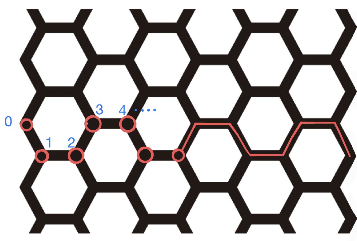
The lattice we are considering is like a “strip” of graphene, means it has finite length in $y$ direction and infinite length in $x$ direction. We may assume that $N$ hexagon is aligning in $y$ direction, gives $N_j = 2N+2$ total atoms in a “unit cell” (this time the unit cell is a large one).
Detail and Code
Label the cells in $x$ direction by index $n$, and atoms in a unit cell by index $j$ (schematic diagram of a 14-sites-unit-cell-case is drawn below), spin-1/2 is still denoted by $\alpha \in \{ \uparrow, \downarrow \}$.
Translation symmetry along $x$ allows us to introduce $k$, such that
\[c_{nj\alpha} = \sum_k c_{kj\alpha} e^{-ikn}\]and
\[c^\dagger_{nj\alpha} = \sum_k c^\dagger_{kj\alpha} e^{ikn}\]first consider the nearest hopping term, by some routine calculation
\[H_1 = t_1 \sum_k \sum_{j} \sum_{\Delta} c^\dagger_{kj\alpha} c_{k(j+\Delta j)\alpha} e^{-i k \Delta n}\]where $\Delta$ goes over the 3 nearest neighbor of each atom, thus for each $k \in [0, 2\pi]$, an effective hamiltonian $h(k)$ in $2N_j \times 2N_j$ matrix form is obtained. For which, the base vector can be chosen as
\[\left[ 0\uparrow, 0 \downarrow, 1\uparrow, 1\downarrow, \dots , Nj-1\uparrow, Nj-1\downarrow \right]\]the matrix element is non-zero only if the electron can transit between two sites
\[h_{j\alpha, (j+\Delta j)\alpha} = t_1 \sum_{\Delta n} e^{-i k \Delta n}\]Code below adds the nearest neighbor hopping term, along with the sub-lattice potential term
def addHopping1(mat, Nj, t1, tr, tv, kx):
    for j in range(Nj):
        if j % 2 == 0:
            # sub-lattice potential
            mat[(2*j, 2*j)] += tv
            mat[(2*j + 1, 2*j + 1)] += tv
            if j % 4 == 0:
                # hoppingTo = {(\Delta n, \Delta j): (\Delta x, \Delta y), ... }
                hoppingTo = {(0, 1): (-0.5, np.sqrt(3)/6), (0, -1): (0, -np.sqrt(3)/3), (1, 1): (0.5, np.sqrt(3)/6)}
            else:
                hoppingTo = {(0, 1): (-0.5, np.sqrt(3)/6), (0, -1): (0, -np.sqrt(3)/3), (-1, 1): (0.5, np.sqrt(3)/6)}
        else:
            mat[(2*j, 2*j)] += -tv
            mat[(2*j + 1, 2*j + 1)] += -tv
            if j % 4 == 1:
                hoppingTo = {(0, 1): (0, np.sqrt(3)/3), (0, -1): (0.5, -np.sqrt(3)/6), (-1, -1): (-0.5, -np.sqrt(3)/6)}
            else:
                hoppingTo = {(0, 1): (0, np.sqrt(3)/3), (0, -1): (0.5, -np.sqrt(3)/6), (1, -1): (-0.5, -np.sqrt(3)/6)}
        for delta in hoppingTo:
            dx, dy = hoppingTo[delta]
            jDes = delta[1] + j
            if jDes >= 0 and jDes < Nj:
                elem = np.exp(-1j * delta[0] * kx)
                # nearest hopping
                mat[(2*j, 2*jDes)] += elem * t1
                mat[(2*j + 1, 2*jDes + 1)] += elem * t1
                # Rashba term
                mat[(2*j+1, 2*jDes)] += 1j * tr * (dy + 1j * dx) * elem
                mat[(2*j, 2*jDes+1)] += 1j * tr * (dy - 1j * dx) * elem
For the second neighbors
def addHopping2(mat, Nj, t2, kx):
    for j in range(Nj):
        if j % 4 == 0:
            des = [(0, 2, -1), (0, -2, -1), (-1, 0, +1), (1, 0, -1), (+1, -2, +1), (+1, 2, +1)]
        elif j % 4 == 1:
            des = [(0, 2, -1), (0, -2, -1), (-1, 0, -1), (1, 0, +1), (-1, -2, +1), (-1, 2, +1)]
        elif j % 4 == 2:
            des = [(0, 2, +1), (0, -2, +1), (-1, 0, +1), (1, 0, -1), (-1, -2, -1), (-1, 2, -1)]
        else:
            des = [(0, 2, +1), (0, -2, +1), (-1, 0, -1), (1, 0, +1), (+1, -2, -1), (+1, 2, -1)]
        for delta in des:
            jDes = delta[1] + j
            if jDes >= 0 and jDes < Nj:
                elem = 1j * delta[2] * t2 * np.exp(-1j * delta[0] * kx)
                mat[(2*j, 2*jDes)] += elem
                mat[(2*j + 1, 2*jDes + 1)] += -elem
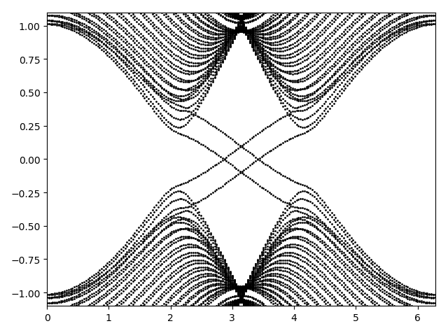
and the output spectrum (in correspondence with ref1)
Discussions
自TKNN number 将第一类陈数引入凝聚态体系后,人们一直试图回答下面几个问题:
- 对于满足时间反演不变的体系,虽然其第一类陈数恒为0,但是否存在其它拓扑不 变量?
- 除了构成集合Z,拓扑数还有无其它可能?
- 可以在三维材料中找到拓扑不变量么?
Kane-Mele 模型提出之前,学界已经从理论和实验上研究了一类绝缘体中的自旋霍尔效应(SHE)。2005 年,在单层石墨烯制备成功的基础上,Kane 与Mele 通过在石墨烯中引入自旋-轨道耦合并建模计算,从理论上提出了一种新的现象——量子自旋霍尔效应(QSHE),并指出了实验上的观测方式2。研究了该模型的边缘态后,他们指出这种QSH 相应当有着非平庸的拓扑性质,可以和之前自旋霍尔效应中涉及的体系区分开来。
然而,由于时间反演(TR) 对称性的存在,陈数并不能用来描述QSH 相体系的拓扑。之后的工作1 中,他们在满足时间反演对称性的二维哈密顿量之上定义了一个新的Z2拓扑不变量。再后来,这一拓扑分类被进一步推广到三维材料,于是,具有TR 对称性的绝缘体,均可采取这种拓扑绝缘体和普通绝缘体的分类法。从而对前述三个问题均给出了肯定的结论。Kane 与Mele 的这项工作,提出了一种实验可测的新现象,推进了TKNN 开创的拓扑物性领域,指导了后续的大量理论与实验,是一项重要的开创性工作。
-
$Z^2$ Topological Order and the Quantum Spin Hall Effect Phys. Rev. Lett. 95, 146802 (2005). ↩ ↩2
-
Quantum Spin Hall Effect in Graphene Phys. Rev. Lett. 95, 226801 (2005). ↩